Components¶

What is a component¶

Components Decomposing signals in components (matrix factorization problems) A very general formulation of the problem can be stated as follows: What could be a function from an m dimensional space to an n dimensional space such that the transformed variables give information on the data that is otherwise hidden in the large data set. That is, the transformed variables should be the underlying factors or components that describe the essential structure of the data. It is hoped that thesecomponents correspond to some physical causes that were involved in the process that generated the data in the first place.

Ben Grossmann (https://math.stackexchange.com/users/81360/ben-grossmann), Is there a geometric meaning to the outer product of two vectors?, URL (version: 2020-04-23): https://math.stackexchange.com/q/965657

For any vector $x$ ,

$uv^T(x)=(v \cdot x)u$

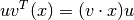
That is, If $u$ and $v$ are unit vectors, $uv^T(x)$ is the component of $x$ in the $v$ direction, taken into the $u$ direction.

QR decomposition¶

see find orthognal vectors

Principal Component Analysis¶

Principal Component Analysis (PCA) is the corner stone of machine learning methods. PCA is map the data to lower dimensional. In order for PCA to do that it should calculate and rank the importance of features/dimensions. There are 2 ways to do so.

using eigenvalue and eigenvector in covariance matrix to calculate and rank the importance of features using SVD on covariance matrix to calculate and rank the importance of the features SVD (covariance matrix) = [U S V’]

https://mathoverflow.net/questions/64579/difference-between-principal-component-analysispca-and-singular-value-decompos

https://intoli.com/blog/pca-and-svd/

https://stats.stackexchange.com/questions/2691/making-sense-of-principal-component-analysis-eigenvectors-eigenvalues

https://www.ece.rutgers.edu/~orfanidi/ece525/svd.pdf

Computing PCs using the covariance method¶

load hald
X=ingredients;
[coeff,score1] = pca(X);

A=X-mean(X);
C=cov(A);
[V,D]=eig(C);
W=fliplr(V);
% score2=(W'*A')';
score2=A*W;

figure;
plot(score1(:,1),score1(:,2),'o')
hold on
plot(score2(:,1),score2(:,2),'x')

Why eigen vector of covariance matrix works¶

The eigenvalues of the covariance matrix encode the variability of the data in an orthogonal basis that captures as much of the data’s variability as possible in the first few basis functions (aka the principle component basis). https://www.mathworks.com/matlabcentral/answers/73298-what-does-eigenvalues-expres-in-the-covariance-matrix

Proof: direction of the greatest variance is eigenvector - Finding the eigen vector of covariance matrix is a way to maximize the variance.

>> data
data =
   -2.2588    0.3188   -0.4336
    0.8622   -1.3077    0.3426

>> X=data'-mean(data')
X =
   -1.4676    0.8965
    1.1100   -1.2734
    0.3576    0.3769

>> cov(X,1)
ans =
    1.1713   -0.8648
   -0.8648    0.8558

>> C=X'*X./3
C =
    1.1713   -0.8648
   -0.8648    0.8558

>> e
e =
    0.2813
    0.9596

>> e'*C*e
ans =
    0.4138

>> sum((X*e).^2)/3
ans =
    0.4138

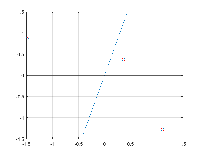
This is a real-data example to show that if we define this vector as $\vec{v}$ , then the projection of our data $D$ onto this vector is obtained as $\vec{v}^{\intercal} D$ , and the variance of the projected data is $\vec{v}^{\intercal} \Sigma \vec{v}$ . Since we are looking for the vector $\vec{v}$ that points into the direction of the largest variance, we should choose its components such that the covariance matrix $\vec{v}^{\intercal} \Sigma \vec{v}$ of the projected data is as large as possible. Maximizing any function of the form $\vec{v}^{\intercal} \Sigma \vec{v}$ with respect to $\vec{v}$ , where $\vec{v}$ is a normalized unit vector, can be formulated as a so called Rayleigh Quotient. The maximum of such a Rayleigh Quotient is obtained by setting $\vec{v}$ equal to the largest eigenvector of matrix $\Sigma$ .

https://www.visiondummy.com/2014/04/geometric-interpretation-covariance-matrix/

Relationship between PCA and SVD¶

PCA and SVD are closely related approaches and can be both applied to decompose any rectangular matrices. We can look into their relationship by performing SVD on the covariance matrix C:

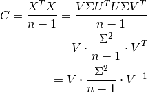
$C = \frac{X^T X}{n-1} = \frac{V \Sigma U^{T} U \Sigma V^{T}}{n-1} \\ = V \cdot \frac{\Sigma^{2}}{n-1} \cdot V^{T} \\ = V \cdot \frac{\Sigma^{2}}{n-1} \cdot V^{-1} \\$

https://towardsdatascience.com/pca-and-svd-explained-with-numpy-5d13b0d2a4d8

Computing PCs using optimization¶

load hald
X=ingredients;
coeff = pca(X);

X=X-mean(X);
[optima]=fminsearch(@i_totlenproj,ones(size(X,2),1),[],X);
optima=optima./norm(optima);
norm(optima-coeff(:,1))

function d=i_totlenproj(u,X)
    d=X*u/norm(u);
    d=-norm(d-d','fro');
end