Regression¶

Machine learning is based upon optimization techniques for data. The goal is to find both a low-rank subspace for optimally embedding the data, as well as regression methods for clustering and classification of different data types. Machine learning thus provides a principled set of mathematical methods for extracting meaningful features from data, i.e. data mining, as well as binning the data into distinct and meaningful patterns that can be exploited for decision making, state estimation and forecasting. Specifically, it learns from and makes predictions based on data. For business applications, this is often called predictive analytics, and it is at the forefront of modern data-driven decision making. In an integrated system, such as is found in autonomous robotics, various machine learning components (e.g., for processing visual and tactile stimulus) can be integrated to form what we now call artificial intelligence (AI). To be explicit: AI is built upon integrated machine learning algorithms, which in turn are fundamentally rooted in optimization. Regression methods are used to find the best model for the given labeled data, via optimization. This model is then used for prediction and classification using new data. There are important variants of supervised methods, including semi-supervised learning in which incomplete training is given so that some of the input/output relationships are missing, i.e. for some input data, the actual output is missing. Active learning is another common subclass of supervised methods whereby the algorithm can only obtain training labels for a limited set of instances, based on a budget, and also has to optimize its choice of objects to acquire labels for. In an interactive framework, these can be presented to the user for labeling. Finally, in reinforcement learning, rewards or punishments are the training labels that help shape the regression architecture in order to build the best model.

Least squares using matrices¶

https://www.youtube.com/watch?v=RlQBEhLhM8Y&list=PLkZjai-2Jcxlg-Z1roB0pUwFU-P58tvOx&index=27

Normal equation solution of the least-squares problem¶

Adopted from https://www.geeksforgeeks.org/ml-normal-equation-in-linear-regression/

Normal Equation in Linear Regression - Normal Equation is an analytical approach to Linear Regression with a Least Square Cost Function. We can directly find out the value of :math’`theta’ without using Gradient Descent. Following this approach is an effective and a time-saving option when are working with a dataset with small features.

The normal equation is as follows:

$\theta = (X^{T}X)^{-1}\cdot(X^{T}y)$

In the above equation, $theta$ is the hypothesis parameters that define it the best, $X$ , input feature value of each instance, and $y$ , output value of each instance. Maths Behind the equation – Given the hypothesis function

$h(\theta)=\theta_{0}x_{0}+\theta_{1}x_{1}+\ldots+\theta_{n}x_{n}$

where, n : the no. of features in the data set. x0 : 1 (for vector multiplication). Notice that this is dot product between θ and x values. So for the convenience to solve we can write it as: $h(\theta)=\theta^{T}x$ .

The motive in Linear Regression is to minimize the cost function:

$\mathrm{J}(\Theta)=\frac{1}{2 m} \sum_{i=1}^{m} \frac{1}{2}\left[h_{\Theta}\left(x^{(i)}\right)-y^{(i)}\right]^{2}$

where, xi : the input value of iih training example. m : no. of training instances n : no. of data-set features yi : the expected result of ith instance

Let us representing cost function in a vector form. This can further be reduced to $X\theta - y$ . But each residual value is squared. We cannot simply square the above expression. As the square of a vector/matrix is not equal to the square of each of its values. So to get the squared value, multiply the vector/matrix with its transpose. So, the final equation derived is

$(X\theta - y)^{T}(X\theta - y)$

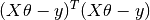
Therefore, the cost function is

$Cost = (X\theta - y)^{T}(X\theta - y)$

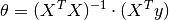
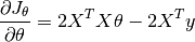
So, now getting the value of θ using derivative

$\frac{\partial J_{\theta}}{\partial \theta}=\frac{\partial}{\partial \theta}\left[(X \theta-y)^{T}(X \theta-y)\right]$

That is

$\frac{\partial J_{\theta}}{\partial \theta}=2X^{T}X\theta - 2X^{T}y$

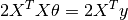
When we set 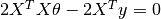$Cost'(\theta)=0$ , i.e., $2X^{T}X\theta - 2X^{T}y = 0$ , we obtain

$2X^{T}X\theta = 2X^{T}y$

In other words,

$(X^{T}X)^{-1}(X^{T}X)\theta = (X^{T}X)^{-1})(X^{T}y)$

Therefore, we obtain the final format

$\theta = (X^{T}X)^{-1}\cdot(X^{T}y)$

So, this is the finally derived Normal Equation with $\theta$ giving the minimum cost value.

Ref: https://eli.thegreenplace.net/2014/derivation-of-the-normal-equation-for-linear-regression/

Gradient Descent for Linear Regression¶

https://youtu.be/B3w5Zzuqi-E?t=449 https://youtu.be/B3w5Zzuqi-E?t=718

LASSO¶

Lasso was originally an acronym for “least absolute shrinkage and selection operator”. Today, lasso is considered a word and not an acronym. Lasso is used for prediction, for model selection, and as a component of estimators to perform inference. Lasso, elastic net, and square-root lasso are designed for model selection and prediction.

Lasso is a method for selecting and fitting covariates that appear in a model. The lasso command can fit linear, logit, probit, and Poisson models. Let’s consider a linear model, a model of y on x1, x2, … , xp. You would ordinarily fit this model by typing

. regress y x1 x2 . . . xp

Now assume that you are uncertain which variables (covariates) belong in the model, although you are certain that some of them do and the number of them is small relative to the number of observations in your dataset, N. In that case, you can type

. lasso linear y x1 x2 . . . xp

You can specify hundreds or even thousands of covariates. You can even specify more covariates than there are observations in your data! The covariates you specify are the potential covariates from which lasso selects.

Lasso is used in three ways: 1. Lasso is used for prediction. 2. Lasso is used for model selection. 3. Lasso is used for inference.

By prediction, we mean predicting the value of an outcome conditional on a large set of potential regressors. And we mean predicting the outcome both in and out of sample. By model selection, we mean selecting a set of variables that predicts the outcome well. We do not mean selecting variables in the true model or placing a scientific interpretation on the coefficients. Instead, we mean selecting variables that correlate well with the outcome in one dataset and testing whether those same variables predict the outcome well in other datasets.

By inference, we mean inference for interpreting and giving meaning to the coefficients of the fitted model. Inference is concerned with estimating effects of variables in the true model and estimating standard errors, confidence intervals, p-values, and the like.

Lasso for prediction¶

Lasso was invented by Tibshirani (1996) and has been commonly used in building models for prediction. Hastie, Tibshirani, and Wainwright (2015) provide an excellent introduction to the mechanics of the lasso and to the lasso as a tool for prediction. See Buhlmann and van de Geer ¨ (2011) for more technical discussion and clear discussion of the properties of lasso under different assumptions. Lasso does not necessarily select the covariates that appear in the true model, but it does select a set of variables that are correlated with them. If lasso selects potential covariate x47, that means x47 belongs in the model or is correlated with variables that belong in the model. If lasso omits potential covariate x52, that means x52 does not belong in the model or belongs but is correlated with covariates that were already selected. Because we are interested only in prediction, we are not concerned with the exact variables selected, only that they are useful for prediction. The model lasso selects is suitable for making predictions in samples outside the one you used for estimation. Everyone knows about the danger of overfitting. Fit a model on one set of data and include too many variables, and the result will exploit features randomly unique to those data that will not be replicated in other data. “Oh,” you may be thinking, “you mean that I can split my data into an estimation sample and a hold-out sample, and after fitting, I can evaluate the model in the hold-out sample.” That is not what we mean, although you can do this, and it is sometimes a good idea to do so. We mean that lasso works to avoid the problem of overfitting by minimizing an estimate of the out-of-sample prediction error.

How lasso for prediction works¶

Lasso finds a solution for

$\mathbf{y}=\beta_{1} \mathbf{x}_{1}+\beta_{2} \mathbf{x}_{2}+\cdots+\beta_{p} \mathbf{x}_{p}+\boldsymbol{\epsilon}$

by minimizing the prediction error subject to the constraint that the model is not too complex—that is, it is sparse. Lasso measures complexity by the sum of the absolute values of β1, β2, … , βp. The solution is obtained by minimizing

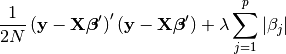
$\frac{1}{2 N}\left(\mathbf{y}-\mathbf{X} \boldsymbol{\beta}^{\prime}\right)^{\prime}\left(\mathbf{y}-\mathbf{X} \boldsymbol{\beta}^{\prime}\right)+\lambda \sum_{j=1}^{p}\left|\beta_{j}\right|$

The first term, (y − Xβ0)(y − Xβ0), is the in-sample prediction error. It is the same value that least squares minimizes.

The second term, λPj|βj |, is a penalty that increases in value the more complex the model. It is this term that causes lasso to omit variables. They are omitted because of the nondifferentiable kinks in the P j|βj | absolute value terms. Had the kinks not been present—think of squared complexity terms rather than absolute value—none of the coefficients would be exactly zero. The kinks cause some coefficients to be zero.

If you minimized (1) with respect to the βj ’s and λ, the solution would be λ = 0. That would set the penalty to zero. λ = 0 corresponds to a model with maximum complexity. Lasso proceeds differently. It minimizes (1) for given values of λ. Lasso then chooses one of those solutions as best based on another criterion, such as an estimate of the out-of-sample prediction error.

When we use lasso for prediction, we must assume the unknown true model contains few variables relative to the number of observations, N. This is known as the sparsity assumption. How many true variables are allowed for a given N? We can tell you that the number cannot be greater than something proportional to √ N / ln q, where q = max{N, p} and p is the number of potential variables. We cannot, however, say what the constant of proportionality is. That this upper bound decreases with q can be viewed as the cost of performing covariate selection.

Lasso provides various ways of selecting λ: CV, adaptive lasso, and a plugin estimator. CV selects the λ that minimizes an estimate of the out-of-sample prediction error. Adaptive lasso performs multiple lassos, each with CV. After each lasso, variables with zero coefficients are removed and remaining variables are given penalty weights designed to drive small coefficients to zero. Thus, adaptive lasso typically selects fewer covariates than CV. The plugin method was designed to achieve an optimal sparsity rate. It tends to select a larger λ than CV and, therefore, fewer covariates in the final model. See [LASSO] lasso and [LASSO] lasso fitting for more information on the methods of selecting λ, their differences, and how you can control the selection process.

Ref: https://www.stata.com/manuals/lassolassointro.pdf

Logistic regression¶

Logistic regression is following :

first we are calculating logit which is equal to

L=b0+b1*x

then we are calculating probability which is equal to p=e^L/(1+e^L)

and finally we are calculating

y*ln(p)+(1-y)*ln(1-p)

function B=logistic_regression(x,y)
  f=@(a)(sum(y.*log((exp(a(1)+a(2)*x)/(1+exp(a(1)+a(2)*x))))+(1-y).*log((1-((exp(a(1)+a(2)*x)/(1+exp(a(1)+a(2)*x))))))));
  a=[0.1, 0.1];
  options = optimset('PlotFcns',@optimplotfval);
  B = fminsearch(f,a, options);
end

In order to implement a logistic regression model, I usually call the glmfit function, which is the simpler way to go. The syntax is:

b = glmfit(x,y,'binomial','link','logit');

b is a vector that contains the coefficients for the linear portion of the logistic regression (the first element is the constant term alpha of the regression). x contains the predictors data, with one row for each observation and one column for each variable. y contains the target variable, usually a vector of boolean (0 or 1) values representing the outcome.

Once you obtain the coefficients, you have to apply the linear part of the regression to your predictors:

z = b(1) + (x * b(2));

To finish, you must apply the logistic function to the output of the linear part:

z = 1 ./ (1 + exp(-z));

https://stackoverflow.com/questions/47247946/logistic-regression-in-matlab