Optimization¶

All of machine learning revolves around optimization. This includes regression and model selection frameworks that aim to provide parsimonious and interpretable models for data. Curve fitting is the most basic of regression techniques, with polynomial and exponential fitting resulting in solutions that come from solving linear systems of equations. This can be generalized for fitting of nonlinear systems. Importantly, regression are typically applied to under- or over-determined systems, thus requiring cross-validation strategies to evaluate the results.

PCA as an optimization problem¶

load hald
X=ingredients;
coeff = pca(X);

X=X-mean(X);
[optima]=fminsearch(@i_totlenproj,ones(size(X,2),1),[],X);
optima=optima./norm(optima);
norm(optima-coeff(:,1))

To run this code we need to define a helper function i_totlenproj:

function d=i_totlenproj(u,X)
    d=X*u/norm(u);
    d=-norm(d-d','fro');
end

i_totlenproj is a cost function or object function. The object of our optimization procedure is to find values in variable u so that the return value of the cost function, d, reaches its minimal.

https://docs.microsoft.com/en-us/azure/quantum/optimization-overview-key-concepts

To understand optimization problems, you first need to learn some basic terms and concepts.

Cost function¶

A cost function is a mathematical description of a problem which, when evaluated, tells you the value of that solution. Typically in optimization problems, we are looking to find the lowest value solution to a problem. In other words, we are trying to minimize the cost.

Search space¶

The search space contains all the feasible solutions to an optimization problem. Each point in this search space is a valid solution to the problem but it may not necessarily be the lowest point, which corresponds to the lowest cost solution.

Optimization landscape Together, the search space and the cost function are often referred to as an optimization landscape. In the case of a problem that involves two continuous variables, the analogy to a landscape is quite direct.

Let’s explore a few different optimization landscapes and see which are good candidates for Azure Quantum optimization.

A smooth, convex landscape¶

Consider the following plot of a cost function that looks like a single smooth valley:

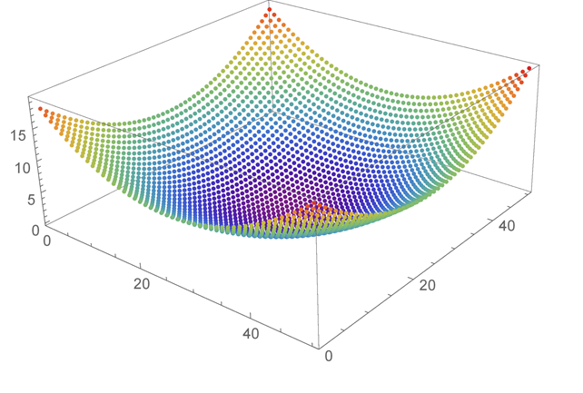
This kind of problem is easily solved with techniques such as gradient descent, where you begin from an initial starting point and greedily move to any solution with a lower cost. After a few moves, the solution converges to the global minimum. The global minimum is the lowest point in the optimization landscape. Azure Quantum optimization solvers offer no advantages over other techniques with these straightforward problems.

A structured, rugged landscape¶

Azure Quantum works best with problems where the landscape is rugged, with many hills and valleys. Here’s an example that considers two continuous variables.

An optimization landscape showing many hills and valleys

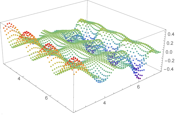
In this scenario, one of the greatest challenges is to avoid getting stuck at any of the sub-optimal local minima. A rugged landscape can have multiple valleys. Each of these valleys will have a lowest point, which is the local minimum. One of these points will be the lowest overall, and that point is the global minimum. These rugged landscapes present situations where Azure Quantum optimization solvers can outperform other techniques.

A scattered, random landscape¶

So far we have discussed smooth and rugged cost functions, but what if there is no structure at all? The following diagram shows such a landscape:

An optimization landscape showing scattered points with no pattern

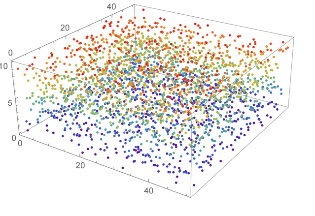
In these cases, where the solutions are completely random, then no algorithm can improve on a brute force search.

Defining a cost function¶

As mentioned above, the cost function represents the quantity that you want to minimize. Its main purpose is to map each configuration of a problem to a single number. This allows the optimizer to easily compare potential solutions and determine which is better. The key to generating a cost function for your problem is in recognizing what parameters of your system affect the chosen cost.

In principle, the cost function could be any mathematical function $f = f(x_0,x_1,\ldots)$ , where the function variables $x_0,x_1,\ldots$ encode the different configurations. The smooth landscape shown above could for example be generated using a quadratic function of two continuous variables $f(x,y) = x^2+y^2$ . However, certain optimization methods may expect the cost function to be in a particular form. For instance, the Azure Quantum solvers expect a Binary Optimization Problem. For this problem type, configurations must be expressed via binary variables with $x_i \in 0,1$ , and many problems are naturally suited to be expressed in this form.

Variables¶

Let’s take a look at how to define the cost function for a simple problem. Firstly, we have a number of variables. We can name these variables x, and if we have i variables, then we can index them individually as follows: .. math:

x_i

For example, if we had 5 variables, we could index like so: .. math:

x_0, x_1, x_2, x_3, x_4

These variables can take specific values, and in the case of a binary optimization problem they can only take two. In particular, if your problem is considering these variables as spins, as in the Ising model, then the values of the variables can be either $+1$ or $-1$ . In other cases, the variables can simply be assigned 1 or 0, as in the Quadratic Unconstrained Binary Optimization (QUBO) or Polynomial Unconstrained Binary Optimization (PUBO) model.

Weights¶

Let us consider some variables. Each of these variables has an associated weight, which determines their influence on the overall cost function.

We can write these weights as $w$ , and again, if we have $i$ variables, then the associated weight for those individual variables can be indexed like this

$w_i$

If we had 5 weights, we could index like this: .. math:

w_1, w_2, w_3, w_4, w_5

A weight can be any real-valued number. For example, we may give these weights the following values:

$w_1=50, w_2=-2, w_3=7, w_4=24, w_5=-10$

Gradient Descent¶

Let’s solve the first example optimization problem. We are going to find the optimized solution to minimize the output value of a function $f(x_1,x_2)=x_1^2 + x_1*x_2 + 3x_2^2$ .

syms x1 x2
f=x1^2+x1*x2+3*x2^2
diff(f,x1)
ans =
   2*x1 + x2
diff(f,x2)
ans =
  x1 + 6*x2

With this informaiton, we can define the gradient of the objective:

function g = grad(x)
  g = [2*x(1)+x(2) x(1)+6*x(2)];
end

Here is the code of the gradient descent algorithm implemented by James T. Allison.

function [xopt,fopt] = grad_descent

  alpha = 0.1;  % step size (0.33 causes instability, 0.2 quite accurate)
  gnorm = inf;  % gradient norm
  x = x0;       % optimization vector
  niter = 0;    % iteration counter
  dx = inf;     % perturbation

  f = @(x1,x2) x1.^2 + x1.*x2 + 3*x2.^2;  % define the objective function:
  f2 = @(x) f(x(1),x(2)); % redefine objective function syntax for use with optimization

  while and(gnorm>=1e-6, and(niter <= 1000, dx >= 1e-6))
      g = grad(x);  % calculate gradient:
      gnorm = norm(g);
      xnew = x - alpha*g;  % take step:
      % check step
      if ~isfinite(xnew)
          display(['Number of iterations: ' num2str(niter)])
          error('x is inf or NaN')
      end
      % update termination metrics
      niter = niter + 1;
      dx = norm(xnew-x);
      x = xnew;
  end

  xopt=x;
  fopt=f2(xopt);
end

The same results should be obtained using fminsearch

f = @(x) x(1).^2 + x(1)*x(2) + 3*x(2).^2;
x0 = [3,3];
xopt = fminsearch(f,x0)
xopt =
 1.0e-04 *
  0.4246   -0.2823

Let’s try another example $f(x_1,x_2,x_3)=4(x_1^2+x_2-x_3)^2+10$

syms x1 x2 x3
f=4*(x1^2+x2-x3)^2+10
diff(f,x1)
ans =
16*x1*(x1^2 + x2 - x3)
diff(f,x2)
ans =
8*x1^2 + 8*x2 - 8*x3
diff(f,x3)
ans =
 - 8*x1^2 - 8*x2 + 8*x3

Therefore, the objective function is defined as the follows:

function g = grad(x)
  g = [16*x(1)*(x(1).^2 + x(2) - x(3)
       8*x(1).^2 + 8*x(2) - 8*x(3)
      -8*x(1).^2 - 8*x(2) + 8*x(3)];
  end

Matlab solution using FMINSEARCH is as follows

f = @(x) 4*(x(1).^2 + x(2)-x(3)).^2 +10;
x0 = [3,3,3];
xopt = fminsearch(f,x0)
xopt =
  0.8911    3.4610    4.2551

For linear regression, the derivatives wrt slope m and intercept c are given in the following format. See https://machinelearningmastery.com/linear-regression-tutorial-using-gradient-descent-for-machine-learning/

L = 0.0001  # The learning Rate
epochs = 1000  # The number of iterations to perform gradient descent

n = float(len(X)) # Number of elements in X

# Performing Gradient Descent
for i in range(epochs):
    Y_pred = m*X + c  # The current predicted value of Y
    D_m = (-2/n) * sum(X * (Y - Y_pred))  # Derivative wrt m
    D_c = (-2/n) * sum(Y - Y_pred)  # Derivative wrt c
    m = m - L * D_m  # Update m
    c = c - L * D_c  # Update c

print (m, c)

Here is how the derivates wrt $m$ and $c$ are computed using Matlab symbolic.

syms x y m c
f=0.5*(y-(m*x+c))^2
f =
  (c - y + m*x)^2/2
diff(f,m)
  ans =
  x*(c - y + m*x)
diff(f,c)
  ans =
  c - y + m*x

Therefore the cost function is:

function g = grad(m,c,X,Y)
  n=length(Y);
  Y_pred = m*X + c;
  D_m = (-2/n) * sum(X * (Y - Y_pred))  % Derivative wrt m
  D_c = (-2/n) * sum(Y - Y_pred)        % Derivative wrt c
  g=[D_m D_c];
end

Ref https://towardsdatascience.com/linear-regression-simplified-ordinary-least-square-vs-gradient-descent-48145de2cf76